Advanced Linear Regression in Python: Math, Code, and Machine Learning Insights [2025 Guide]
If you’re brand new, pause here 👉 Linear Regression Basics in Machine Learning (Beginner’s Guide 2025). That’s where regression starts simple — just one line, one variable, and one prediction. Now, we go beyond the basics into Advanced Linear Regression in Python — where math meets code, and where theory becomes machine learning practice.
Linear regression in machine learning is all about predicting continuous outcomes. Salary based on years of experience. House price based on square footage. Stock return based on market index. Simple but powerful.
Think of it as drawing the “best possible straight line” through data points so you can predict tomorrow using yesterday’s trends.
Now, let’s peel back the layers and go from basics → advanced.
🔥 Key Highlights
📉 Cost Function & Gradient Descent — how linear regression learns by minimizing error.
📊 Multiple Linear Regression — formulas, examples, graphs, and real-world models.
⚖️ Assumptions & Homoscedasticity — why model validity depends on these checks.
🧩 Regularization (Lasso, Ridge, Elastic Net) — handling multicollinearity and overfitting.
🐍 Linear Regression with Python & scikit-learn — step-by-step code examples.
📏 Evaluation Metrics — MAE, RMSE, and R² explained with intuition.
💡 Advantages vs Limitations — when to use regression and when to avoid it.
🚀 Next Steps in ML — how regression connects to advanced algorithms.
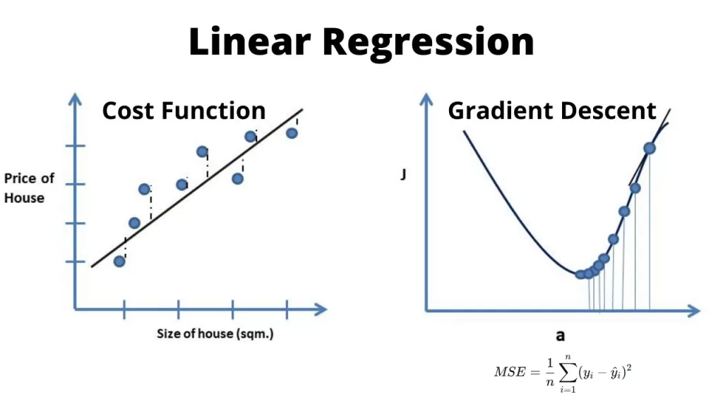
Cost Function in Linear Regression – The Heart of Regression
Every regression model has one question to answer: How wrong am I?
That’s where the cost function in linear regression comes in. The most common one is
Mean Squared Error (MSE)
\( \displaystyle
\text{MSE} \;=\; \frac{1}{n} \sum_{i=1}^{n} \left(y_{i} – \hat{y}_{i}\right)^{2}
\)
\(y_i\)
= actual value (target) for sample i
\(\hat{y}_i\)
= predicted value for sample i (model output)
\(n\)
= number of samples (dataset size)
Tip: MSE squares the error so larger mistakes are penalized more. If you prefer a less-sensitive metric, consider MAE (Mean Absolute Error).
Imagine plotting errors as a curve. You’ll see a parabola-shaped bowl. The bottom of that bowl is the sweet spot — the lowest error, the “best fit.”
💡 Developer Insight: Why squared error, not absolute error?
- Squaring amplifies large mistakes, which is exactly what you want in most cases.
- Absolute error (MAE) is less punishing but trickier to optimize mathematically.
This is why MSE became the default cost function. It gives the math nice properties (smooth, differentiable), making optimization possible.
Gradient Descent in Linear Regression 🚀
Once you define the cost function, the next challenge is how to minimize it. Enter: gradient descent in linear regression.
🚀 Gradient Descent Update Rule
\( \theta = \theta – \alpha \cdot \nabla J(\theta) \)
- \(\theta\) = model parameters (weights)
- \(\alpha\) = learning rate (step size)
- \(J(\theta)\) = cost function
⚡ Too high learning rate overshoots, too low makes training painfully slow.
Picture this: you’re standing somewhere on that error parabola. You want to reach the bottom. Gradient descent tells you which way is downhill and how big a step to take. Step by step, you inch toward the minimum.
⚡ Learning rate pitfalls:
- Too high → you overshoot, bouncing around without settling.
- Too low → you crawl, wasting time.
👉 Interview Tip: FAANG recruiters love to ask: “Explain gradient descent in simple terms.” Answer with the “hill climbing in reverse” analogy, and you’ll stand out.
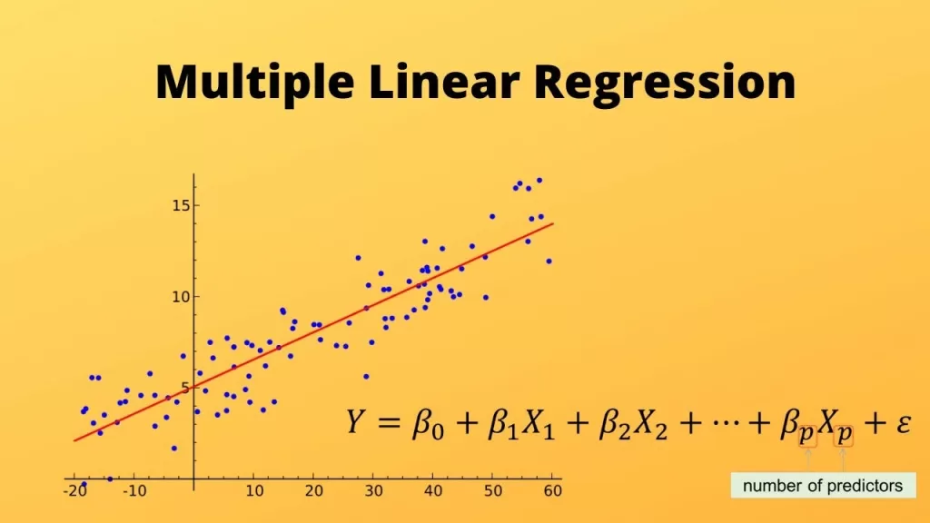
Multiple Linear Regression in Machine Learning
So far, one line → one variable → one prediction. But the real world? Rarely that simple.
That’s where multiple linear regression in machine learning comes in. The formula expands:
📊 Multiple Linear Regression
\( y = \beta_0 + \beta_1 x_1 + \beta_2 x_2 + \cdots + \beta_n x_n \)
- \(\beta_0\) = intercept
- \(\beta_1 \dots \beta_n\) = weights for each feature
- \(x_1 \dots x_n\) = independent variables
🏠 Example: Predicting house price from square footage, location, and number of rooms.
👉 What is multiple linear regression? It’s just regression with more than one input variable. Instead of predicting house price from only square footage, you add location, number of rooms, and age of the building. More features → richer model.
Multiple Linear Regression Example 🏠
A real estate company wants to predict house prices.
- Input features: square footage, location score, number of rooms.
- Output: predicted price.
- Visual: each new feature adds another dimension — the model draws a “hyperplane,” not just a line.

Assumptions of Linear Regression (Must Know 🚨)
Multiple linear regression works best when these hold:
- Linearity → Relationship between inputs and output should be straight-ish.
- No Multicollinearity → Features shouldn’t be highly correlated (or coefficients get unstable).
- Homoscedasticity in linear regression → Residuals (errors) should have constant variance.
- Normality of Residuals → Residuals should follow a normal distribution (important for inference).
👉 Developer Note: Violating assumptions doesn’t always break the model, but it can make predictions unreliable. Always check residual plots before trusting results.

📊 A multiple linear regression graph often shows predicted vs. actual values. If points cluster around the 45° line, your model’s doing well.
Regularization – Taming Overfitting 🔧
Real-world data is messy. Add too many features, and your regression model starts to memorize instead of generalizing. That’s overfitting. Regularization fixes this by adding a penalty to large coefficients.
📊 Regularization Techniques in Linear Regression
| Technique | Formula (Penalty Term) | Best Use Case | Drawback |
|---|---|---|---|
| Ridge Regression (L2) | \( \lambda \sum \beta^2 \) | Handles multicollinearity well | Doesn’t shrink coefficients to zero |
| Lasso Regression (L1) | \( \lambda \sum |\beta| \) | Feature selection (shrinks some coefficients to zero) | Can struggle with highly correlated features |
| Elastic Net Regression | \( \lambda_1 \sum |\beta| + \lambda_2 \sum \beta^2 \) | Balanced trade-off between Ridge and Lasso | Needs extra tuning (two hyperparameters) |
🔑 Quick take:
- Use Ridge when you’ve got many correlated features.
- Use Lasso when you want a simpler model with fewer predictors.
- Use Elastic Net when you can’t decide — it balances both worlds.
Developer insight: In Kaggle competitions, Lasso often gets used for feature selection, then Ridge for fine-tuning the final model. Elastic Net shows up when datasets are wide (tons of features) but noisy.
Python: Linear Regression from Scratch ✍️
You can learn regression theory all day, but nothing sticks like writing the code yourself. Let’s build linear regression from scratch with NumPy before moving to sklearn linear regression.
Gradient Descent Implementation (NumPy)
import numpy as np

# Sample dataset
X = np.array([1, 2, 3, 4, 5])
y = np.array([3, 4, 2, 5, 6])

# Initialize parameters
m, b = 0, 0
learning_rate = 0.01
epochs = 1000
n = len(X)

for _ in range(epochs):
    y_pred = m*X + b
    # Gradients
    Dm = (-2/n) * sum(X * (y - y_pred))
    Db = (-2/n) * sum(y - y_pred)
    # Update
    m -= learning_rate * Dm
    b -= learning_rate * Db

print(f"Final slope: {m}, Intercept: {b}")
👉 This loop shows how weights update step by step. That’s gradient descent in action.
sklearn Linear Regression Example (Production-Ready)
from sklearn.linear_model import LinearRegression
import numpy as np

X = np.array([[1], [2], [3], [4], [5]])
y = np.array([3, 4, 2, 5, 6])

model = LinearRegression()
model.fit(X, y)

print("Slope:", model.coef_[0])
print("Intercept:", model.intercept_)
💡 Difference:
- From scratch = you learn the math, control every detail.
- Sklearn linear regression = fast, reliable, scalable. Ideal for real projects.
Evaluation Metrics 📊
Once you’ve trained your model, the next question is: how good is it? That’s where evaluation metrics in regression come in.
Common Metrics
📏 Mean Absolute Error (MAE)
\( \text{MAE} = \frac{1}{n} \sum |y_i – \hat{y}_i| \)
👍 Easy to interpret — average error in real-world units.
Easy to interpret — the average error in real-world units.
- Root Mean Squared Error (RMSE)
📐 Root Mean Squared Error (RMSE)
\( \text{RMSE} = \sqrt{ \frac{1}{n} \sum (y_i – \hat{y}_i)^2 } \)
🔎 Penalizes big mistakes more. Useful when large errors are costly.
Penalizes big mistakes more. Often preferred when large errors are costly.
- R² Score (Coefficient of Determination)
🎯 R² Score (Coefficient of Determination)
\( R^2 = 1 – \frac{SS_{res}}{SS_{tot}} \)
📊 Tells how much variance in the target is explained by the model.
Measures how much variance in the target your model explains.
sklearn Implementation
from sklearn.metrics import mean_absolute_error, mean_squared_error, r2_score
import numpy as np

y_true = np.array([3, 4, 5, 6, 7])
y_pred = np.array([2.8, 4.1, 4.9, 6.2, 6.8])

print("MAE:", mean_absolute_error(y_true, y_pred))
print("RMSE:", mean_squared_error(y_true, y_pred, squared=False))
print("R²:", r2_score(y_true, y_pred))
💡 Developer Note: Don’t rely only on R². A high R² doesn’t always mean the model is good — sometimes it just means your dataset is tricky or your features are correlated. Always pair R² with MAE or RMSE.
Advantages & Limitations
Linear regression has been around for over 200 years — and for good reason. Even in 2025, companies still use it despite the buzz around deep learning. Why? Because sometimes, you don’t need a spaceship when a bicycle will do the job.
✅ Advantages
- Simplicity → Easy to implement, quick to train.
- Interpretability → Coefficients directly show how each feature affects the outcome.
- Speed → Works on massive datasets without burning GPUs.
- Baseline Model → Great starting point before moving to complex algorithms.
⚠️ Limitations
- Non-linearity → Struggles when relationships aren’t straight lines.
- Outliers → A single extreme value can skew predictions heavily.
- Assumptions → Multiple linear regression assumptions like homoscedasticity in linear regression and no multicollinearity are often violated in messy real-world data.
- Not Always Flexible → Complex patterns (like interactions or curves) require advanced methods or transformations.
💡 Real-world note: A fintech startup might still choose linear regression over neural networks because it’s easier to explain to regulators. Transparency can matter more than accuracy.

Conclusion + Next Steps
You’ve just explored Advanced Linear Regression in Python — from cost functions and gradient descent to multiple regression, regularization, and evaluation metrics. That’s a big leap from drawing a single line through data points.
But here’s the thing: regression isn’t just math on a whiteboard. It’s one of the most battle-tested tools in data science. Banks use it to predict credit risk. Marketing teams use it to measure campaign ROI. Real-estate firms use it to price properties. If you understand regression deeply, you understand one of the pillars of machine learning.
👉 Your Next Steps:
- Interview Prep: Be ready to explain the difference between simple linear regression and multiple linear regression. It’s a classic.
- Skill Upgrade: Try implementing regularization (Lasso, Ridge, Elastic Net) on a dataset you care about. You’ll learn more by tweaking real data than by reading theory.
- Broaden Your ML Toolkit: 🔗 Related Reads You’ll Love
- 🌳 Trees in Data Structures Explained: 5 Must-Know Types, Traversals & a FREE Cheat Sheet (Download Now!)
- 🌲 Mastering Decision Tree in Machine Learning: Step-by-Step Guide with Examples
- 🤖 Machine Learning Algorithms: A Complete Guide for Beginners
- 🔍 What is Linear Search and Binary Search (2025 Guide): Search Algorithms Explained, Code in Python & Java, and More
- ⚡ Binary Searching Algorithm – A Complete Guide to Efficient Searching Algorithms
- 📘 Design and Analysis of Algorithms – A Complete Guide
- 📚 Data Structures and Algorithms: From Basics to Advanced
- 🎯 Support Vector Machines (SVM): My 7 Biggest Takeaways for AI Learners
🚀 Think of regression as your first language in machine learning. Once you master it, every other algorithm — trees, SVMs, neural networks — will make more sense. You’ve built the foundation. Now it’s time to construct the skyscraper.
❓ FAQ: Advanced Linear Regression in Python
Q1. What is multiple linear regression?
Multiple linear regression is an extension of simple regression that uses two or more independent variables to predict a continuous outcome. Example: predicting house prices based on size, location, and number of rooms.
Q2. What’s the difference between simple linear regression and multiple linear regression?
- Simple: one predictor → one outcome.
- Multiple: many predictors → one outcome.
More predictors usually improve accuracy but add complexity.
Q3. What are the main assumptions of linear regression?
- Linearity of relationships.
- No or low multicollinearity.
- Homoscedasticity in linear regression (errors have constant variance).
- Normally distributed residuals.
Q4. When should you not use linear regression?
- When relationships are highly non-linear.
- When data has heavy outliers.
- When key assumptions are violated.
In such cases, tree-based or non-linear models may perform better.
Q5. Why do many companies still use regression in 2025?
Because it’s transparent, explainable, and fast. In finance, healthcare, and law — where decisions need justification — a linear model is often preferred over a black-box neural network.