7 Easy Steps: How to Use VLOOKUP in Excel for Quick Data Lookup ✨

Looking for a fast and effective way to find information in your spreadsheet? You’re in the right place! In this guide, we’ll walk you through how to use VLOOKUP in Excel for quick data lookup. Whether you’re a student, professional, or just someone dealing with lots of data, mastering the Excel VLOOKUP formula will save you tons of time and effort.
📅 Key Highlights:
- Learn how to use VLOOKUP in Excel for quick data lookup with clear, step-by-step instructions.
- Understand the Excel VLOOKUP formula syntax and structure.
- Get real-life examples to boost your learning.
- Discover common VLOOKUP errors and how to fix them.
- Bonus: Tips to enhance your Excel efficiency!
💡 What is VLOOKUP in Excel?
The VLOOKUP function in Excel is a powerful tool used to search for a value in the first column of a range or table and return a value in the same row from another column. It stands for Vertical Lookup.
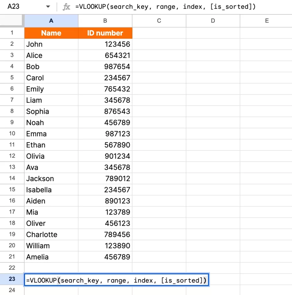
Syntax:
VLOOKUP(lookup_value, table_array, col_index_num, [range_lookup])

Parameters:
- lookup_value: The value you want to search for.
- table_array: The range of cells that contains the data.
- col_index_num: The column number from which the value should be returned.
- range_lookup: TRUE for approximate match, FALSE for exact match.
🔢 Step-by-Step: How to Use VLOOKUP in Excel for Quick Data Lookup
Step 1: Organize Your Data
Ensure your data is arranged in a vertical table where the value to look up is in the first column.
Step 2: Insert the VLOOKUP Formula
In the cell where you want the result, type:
=VLOOKUP("John", A2:C10, 2, FALSE)
This will look for “John” in the first column of range A2:C10 and return the value from the second column.
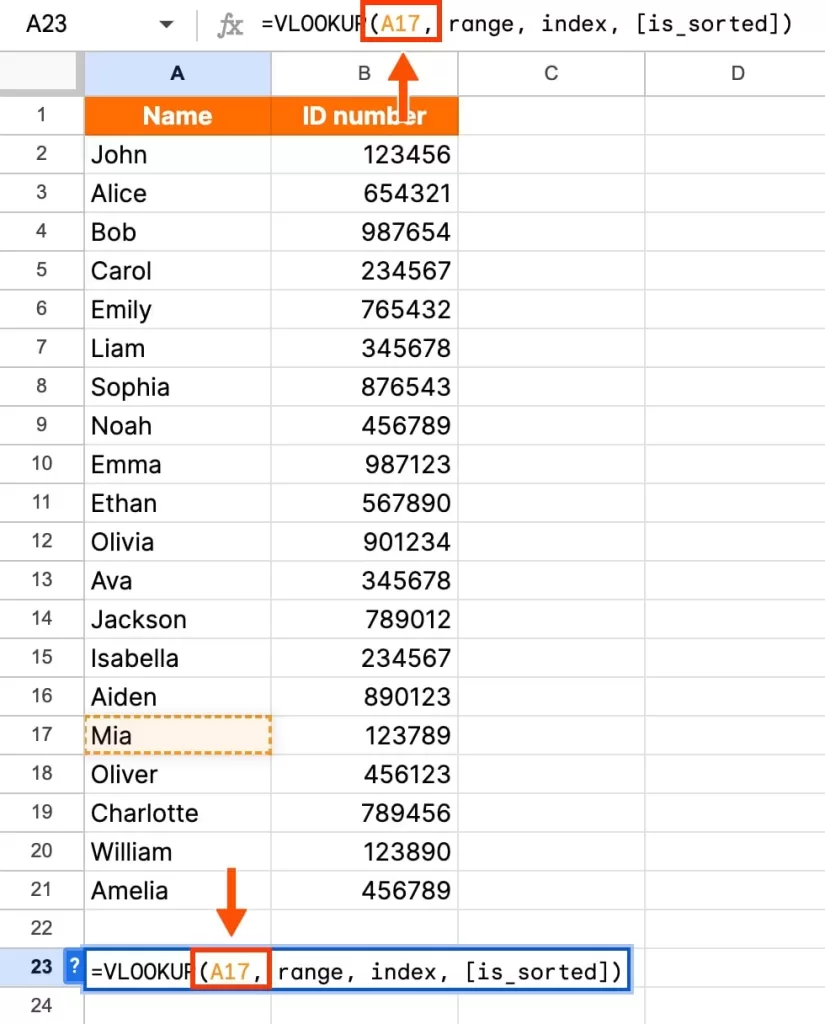
Step 3: Use Cell References
Instead of typing the value directly, you can use a cell reference:
=VLOOKUP(E2, A2:C10, 2, FALSE)
Step 4: Adjust Column Index
Change the column index to return different data:
=VLOOKUP(E2, A2:C10, 3, FALSE)
Step 5: Understand TRUE vs FALSE
- FALSE gives an exact match.
- TRUE returns an approximate match (must be sorted).
Step 6: Use Error Handling
To avoid errors like #N/A:
=IFERROR(VLOOKUP(E2, A2:C10, 2, FALSE), "Not Found")
Step 7: Test with Real Data
Try it out with your own spreadsheet to solidify your understanding.
🤔 Common VLOOKUP Errors and Fixes
- #N/A Error: The value isn’t found. Double-check your data and spelling.
- #REF! Error: The column index is too high.
- Wrong Results: Check if you used TRUE instead of FALSE.

🌟 Excel VLOOKUP Formula Use Cases
- Searching for employee details from an ID
- Getting product prices from a catalog
- Finding student grades
- Auto-filling customer info in forms
Need more Excel help? Check out our guide on Excel Tips for Beginners 🚀
📈 Tips to Improve Your Excel Skills
- Learn XLOOKUP, the newer and more flexible alternative.
- Use Named Ranges for clarity.
- Combine IF + VLOOKUP for advanced logic.
Want to explore more formulas? Visit our article on Top Excel Formulas Every User Should Know!
🌐 Related Reading
📖 Final Thoughts
Now that you’ve learned how to use VLOOKUP in Excel for quick data lookup, you’re ready to tackle spreadsheets with confidence. The Excel VLOOKUP formula is an essential tool that will simplify your data tasks and boost productivity.
So go ahead – try it out, experiment, and see how much time you can save! ✨
If you found this guide helpful, don’t forget to share it with your team or on social media – someone else might need this Excel boost too! 😊