Dijkstra Algorithm Explained with Code & Examples

You know how Google Maps tells you the fastest way to get from point A to point B?

That’s Dijkstra algorithm in action. Well, sort of. It’s behind many shortest path calculations, and it’s the foundation of modern pathfinding tools. When I first learned about it in college, I honestly had no clue what was going on. A bunch of nodes? Edges? Weights? Sounds more like gym equipment than computer science. 😅

But once I saw it in action, it clicked. And today, I’m breaking it down — in plain English — for you.

So if you’re curious about how computers figure out the most efficient path in a weighted graph using a greedy algorithm, let’s dive in.

🚦 What is Dijkstra Algorithm?

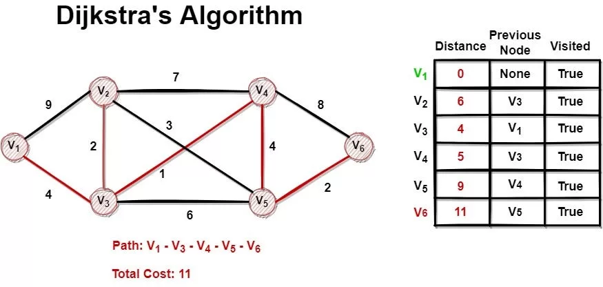
Let me say it again: Dijkstra algorithm helps you find the shortest path between two nodes in a weighted graph (where each edge has a “cost” or “distance”).

If you’re currently exploring a data structures and algorithms course, understanding Dijkstra’s algorithm is a must — it’s one of the most essential concepts you’ll encounter in technical interviews and competitive programming.

🔑 The catch? All edge weights must be non-negative. That means no “reverse tunnels” or “shortcuts” that reward you with negative points.

It’s called a greedy algorithm because it always picks the “closest” unvisited node. It doesn’t overthink — it just grabs the best option right now. Simple, right?

🧭 Real-World Uses of Dijkstra Algorithm

Let’s get practical. Here’s where you’ve already seen Dijkstra in action:

GPS apps (Google Maps, Waze): find shortest driving or walking paths.
Network routing protocols like OSPF (Open Shortest Path First).
Video games (AI enemy pathfinding).
Logistics & supply chain: route optimization for delivery trucks.
Urban planning tools: best infrastructure layouts.

Every time you find an optimized route, there’s a high chance Dijkstra’s algorithm (or one of its cousins) had a say.

🧠 Key Concepts You Need to Know First

Before we jump to code, let’s break down some terms:

Weighted graph: A network of nodes (points) and edges (paths) where each edge has a weight (distance, time, cost).
Greedy algorithm: Chooses the best immediate option without thinking too far ahead.
Priority queue: A data structure that always lets you access the smallest weight node quickly.
Visited nodes: Once a node’s shortest path is found, we don’t revisit it.

✍️ Dijkstra Pseudocode (Algorithm)

Here’s a simplified version of Dijkstra’s pseudocode:

1. Mark all nodes unvisited. Set distance to all nodes as infinity.

2. Set starting node’s distance to 0.

3. While there are unvisited nodes:

a. Choose the unvisited node with the smallest distance.

b. For each neighbor of this node:

– Calculate tentative distance through this node.

– If it’s smaller, update the neighbor’s distance.

c. Mark the node as visited.

4. Done when all nodes are visited or destination reached.

Think of it like exploring a city. You visit the closest block, update routes for nearby places, and move on.

🧪 Python Code Example Using heapq

import heapq

def dijkstra(graph, start):
    distances = {node: float('inf') for node in graph}
    distances[start] = 0
    queue = [(0, start)]

    while queue:
        current_distance, current_node = heapq.heappop(queue)

        for neighbor, weight in graph[current_node]:
            distance = current_distance + weight
            if distance < distances[neighbor]:
                distances[neighbor] = distance
                heapq.heappush(queue, (distance, neighbor))

    return distances

Try it with a graph like this:

graph = {
  'A': [('B', 1), ('C', 4)],
  'B': [('C', 2), ('D', 5)],
  'C': [('D', 1)],
  'D': []
}

Run dijkstra(graph, ‘A’) and it returns shortest distances from A.

This example is written in Python, but you can also implement Dijkstra’s algorithm in Java — something we often teach in our Java course in Chennai and Python course in Chennai, where students build real-time graph applications.

📊 Time Complexity — How Efficient is It?

Let’s talk performance:

Implementation	Time Complexity
Using arrays	O(V²)
Using min-heap (heapq)	O(E log V)

That’s why priority queues (like Python’s heapq) matter.

⚔️ Dijkstra vs Bellman-Ford vs A*

So when shouldn’t you use Dijkstra’s algorithm?

If your graph has negative weights, skip Dijkstra. Use Bellman-Ford.
If you’re optimizing for both speed and accuracy, check out A* (which adds a heuristic).
For all-pairs shortest paths, look at Floyd-Warshall.

❗ Limitations of Dijkstra Algorithm

🚫 No negative weights
🐢 Can be slow on massive graphs (use A* with heuristics or bidirectional Dijkstra)
❌ Doesn’t guarantee the best route in weighted graphs with weird constraints

💡 Final Thoughts

I hope this breakdown of Dijkstra algorithm helps you not just memorize it — but understand it.

Whether you’re prepping for a coding interview, optimizing a project, or just love how algorithms mimic the real world — this one’s a must-know.

Want to master these concepts hands-on? Consider enrolling in a practical data structures and algorithms course or boost your programming skills with our Java or Python courses in Chennai.