We can easily understand above formula using below diagram. Since B has already happened, the sample space reduces to B. So the probability of A happening becomes P(A ∩ B) divided by P(B)

Below is Bayes’s formula for conditional probability.
![]()
The formula provides relationship between P(A|B) and P(B|A). It is mainly derived form conditional probability formula discussed in the previous post.
Consider the below forrmulas for conditional probabilities P(A|B) and P(B|A)
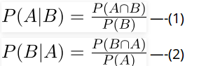
Since P(B ∩ A) = P(A ∩ B), we can replace P(A ∩ B) in first formula with P(B|A)P(A)
After replacing, we get the given formula. Refer this for examples of Bayes’s formula.
A random variable is actually a function that maps outcome of a random event (like coin toss) to a real value.
Coin tossing game :
A player pays 50 bucks if result of coin
toss is "Head"

The person gets 50 bucks if the result is
Tail.

A random variable profit for person can
be defined as below :

Profit = +50 if Head
         -50 if Tail

Generally gambling games are not fair for players,
the organizer takes a share of profit for all
arrangements. So expected profit is negative for
a player in gambling and positive for the organizer.
That is how organizers make money.
Expected value of a random variable R can be defined as following
    E[R] = r1*p1 + r2*p2 + ... rk*pk

    ri ==> Value of R with probability pi
Expected value is basically sum of product of following two terms (for all possible events)
a) Probability of an event.
b) Value of R at that even
Example 1:
In above example of coin toss,
Expected value of profit = 50 * (1/2) +
                          (-50) * (1/2)
                         = 0

Example 2:
Expected value of six faced dice throw is
  = 1*(1/6) + 2*(1/6) + .... + 6*(1/6)
  = 3.5
Let R1 and R2 be two discrete random variables on some probability space, then
E[R1 + R2] = E[R1] + E[R2]
For example, expected value of sum for 3 dice throws is = 3 * 7/2 = 7
Refer this for more detailed explanation and examples.
If probability of success is p in every trial, then expected number of trials until success is 1/p. For example, consider 6 faced fair dice is thrown until a ‘5’ is seen as result of dice throw. The expected number of throws before seeing a 5 is 6. Note that 1/6 is probability of getting a 5 in every trial. So number of trials is 1/(1/6) = 6.
As another example, consider a QuickSort version that keeps on looking for pivots until one of the middle n/2 elements is picked. The expected time number of trials for finding middle pivot would be 2 as probability of picking one of the middle n/2 elements is 1/2. This example is discussed in more detail in Set 1.
Refer this for more detailed explanation and examples. [ad type=”banner”]


