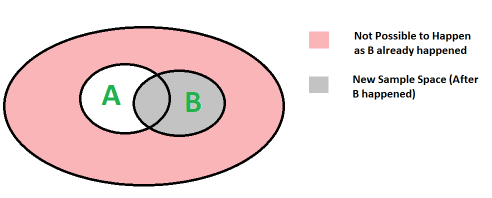
We can easily understand above formula using below diagram. Since B has already happened, the sample space reduces to B. So the probability of A happening becomes P(A ∩ B) divided by P(B)
Below is Bayes’s formula for conditional probability.
![]()
The formula provides relationship between P(A|B) and P(B|A). It is mainly derived form conditional probability formula discussed in the previous post.
Consider the below forrmulas for conditional probabilities P(A|B) and P(B|A)
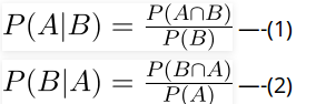
Since P(B ∩ A) = P(A ∩ B), we can replace P(A ∩ B) in first formula with P(B|A)P(A)
After replacing, we get the given formula. Refer this for examples of Bayes’s formula.
A random variable is actually a function that maps outcome of a random event (like coin toss) to a real value.
Example :
Coin tossing game :
A player pays 50 bucks if result of coin
toss is "Head"

The person gets 50 bucks if the result is
Tail.

A random variable profit for person can
be defined as below :

Profit = +50 if Head
         -50 if Tail

Generally gambling games are not fair for players,
the organizer takes a share of profit for all
arrangements. So expected profit is negative for
a player in gambling and positive for the organizer.
That is how organizers make money.
[ad type=”banner”]
Expected value of a random variable R can be defined as following
    E[R] = r1*p1 + r2*p2 + ... rk*pk

    ri ==> Value of R with probability pi
Expected value is basically sum of product of following two terms (for all possible events)
a) Probability of an event.
b) Value of R at that even
Example 1:
In above example of coin toss,
Expected value of profit = 50 * (1/2) +
                          (-50) * (1/2)
                         = 0

Example 2:
Expected value of six faced dice throw is
  = 1*(1/6) + 2*(1/6) + .... + 6*(1/6)
  = 3.5
Let R1 and R2 be two discrete random variables on some probability space, then
E[R1 + R2] = E[R1] + E[R2]
For example, expected value of sum for 3 dice throws is = 3 * 7/2 = 7
Refer this for more detailed explanation and examples.
[ad type=”banner”]If probability of success is p in every trial, then expected number of trials until success is 1/p. For example, consider 6 faced fair dice is thrown until a ‘5’ is seen as result of dice throw. The expected number of throws before seeing a 5 is 6. Note that 1/6 is probability of getting a 5 in every trial. So number of trials is 1/(1/6) = 6.
As another example, consider a QuickSort version that keeps on looking for pivots until one of the middle n/2 elements is picked. The expected time number of trials for finding middle pivot would be 2 as probability of picking one of the middle n/2 elements is 1/2. This example is discussed in more detail in Set 1.
Refer this for more detailed explanation and examples.
- Randomized Algorithms | Set 1 (Introduction and Analysis)
- Randomized Algorithms | Set 2 (Classification and Applications)
- Randomized Algorithms | Set 3 (1/2 Approximate Median)
All Randomized Algorithm Topics
This article is contributed by Shivam Gupta. Please write comments if you find anything incorrect, or you want to share more information about the topic discussed above
[ad type=”banner”]

